Customizing a Pivot Table in Excel 2016

This chapter from Excel 2016 Pivot Table Data Crunching covers how you can use many powerful settings to tweak pivot tables. These tweaks range from making cosmetic changes to changing the underlying calculation used in the pivot table.

In This Chapter                                                                         

1. In This Chapter
2. Making Common Cosmetic Changes
3. Making Report Layout Changes
4. Customizing a Pivot Table’s Appearance with Styles and Themes
5. Changing Summary Calculations
6. Adding and Removing Subtotals
7. Changing the Calculation in a Value Field

Making Common Cosmetic Changes

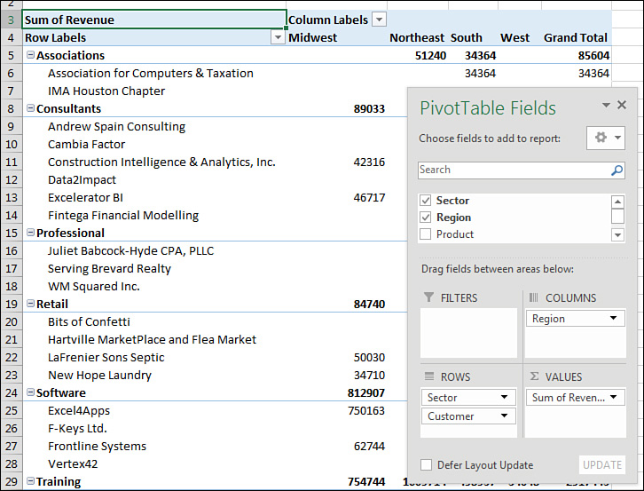
You need to make a few changes to almost every pivot table to make it easier to understand and interpret. Figure 3.1 shows a typical pivot table. To create this pivot table, open the Chapter 3 data file. Select Insert, Pivot Table, OK. Check the Sector, Customer, and Revenue fields, and drag the Region field to the Columns area.

Figure 3.1 A typical pivot table before customization.

This default pivot table contains several annoying items that you might want to change quickly:

• The default table style uses no gridlines, which makes it difficult to follow the rows and columns across and down.
• Numbers in the Values area are in a general number format. There are no commas, currency symbols, and so on.
• For sparse data sets, many blanks appear in the Values area. The blank cell in B5 indicates that there were no Associations sales in the Midwest. Most people prefer to see zeros instead of blanks.
• Excel renames fields in the Values area with the unimaginative name Sum of Revenue. You can change this name.

You can correct each of these annoyances with just a few mouse clicks. The following sections address each issue.

Applying a Table Style to Restore Gridlines

The default pivot table layout contains no gridlines and is rather plain. Fortunately, you can apply a table style. Any table style that you choose is better than the default.

Follow these steps to apply a table style:

1. Make sure that the active cell is in the pivot table.
2. From the ribbon, select the Design tab. Three arrows appear at the right side of the PivotTable Style gallery.
3. Click the bottom arrow to open the complete gallery, which is shown in Figure 3.2.
   

1. Figure 3.2 The gallery contains 85 styles to choose from.
2. Choose any style other than the first style from the drop-down. Styles toward the bottom of the gallery tend to have more formatting.
3. Select the check box for Banded Rows to the left of the PivotTable Styles gallery. This draws gridlines in light styles and adds row stripes in dark styles.

It does not matter which style you choose from the gallery; any of the 84 other styles are better than the default style.

Changing the Number Format to Add Thousands Separators

If you have gone to the trouble of formatting your underlying data, you might expect that the pivot table will capture some of this formatting. Unfortunately, it does not. Even if your underlying data fields were formatted with a certain numeric format, the default pivot table presents values formatted with a general format. As a sign of some progress, when you create pivot tables from PowerPivot, you can specify the number format for a field before creating the pivot table. This functionality has not come to regular pivot tables yet.

For example, in the figures in this chapter, the numbers are in the thousands or tens of thousands. At this level of sales, you would normally have a thousands separator and probably no decimal places. Although the original data had a numeric format applied, the pivot table routinely formats your numbers in an ugly general style.

CAUTION                                                                    

 You will be tempted to format the numbers using the right-click menu and choosing Number Format. This is not the best way to go. You will be tempted to format the cells using the tools on the Home tab. This is not the way to go. Either of these methods temporarily fixes the problem, but you lose the formatting as soon as you move a field in the pivot table. The right way to solve the problem is to use the Number Format button in the Value Field Settings dialog.

You have three ways to get to this dialog:

• Right-click a number in the Values area of the pivot table and select Value Field Settings.
• Click the drop-down to the right of the Sum of Revenue field in the areas of the PivotTable Fields list and then select Value Field Settings from the context menu.
• Select any cell in the Values area of the pivot table. From the Analyze tab, select Field Settings from the Active Field group.

As shown in Figure 3.3, the Value Field Settings dialog is displayed. To change the numeric format, click the Number Format button in the lower-left corner.

Figure 3.3 Display the Value Field Settings dialog, and then click Number Format.

In the Format Cells dialog that appears, you can choose any built-in number format or choose a custom format. For example, you can choose Currency, as shown in Figure 3.4.

Figure 3.4 Choose an easier-to-read number format from the Format Cells dialog.

NOTE                                                                  

Although Excel 2016 offers a Live Preview feature for many formatting settings, the Format Cells dialog does not offer one. To see the changes, you must assign the number format, close the Format dialog, and then close the Value Field Settings dialog.

Replacing Blanks with Zeros

One of the elements of good spreadsheet design is that you should never leave blank cells in a numeric section of a worksheet. Even Microsoft believes in this rule; if your source data for a pivot table contains one million numeric cells and one blank cell, Excel 2016 treats the entire column as if it is text and chooses to count the column instead of sum it. This is why it is incredibly annoying that the default setting for a pivot table leaves many blanks in the Values area of some pivot tables.

A blank tells you that there were no sales for a particular combination of labels. In the default view, an actual zero is used to indicate that there was activity, but the total sales were zero. This value might mean that a customer bought something and then returned it, resulting in net sales of zero. Although there are limited applications in which you need to differentiate between having no sales and having net zero sales, this seems rare. In 99% of the cases, you should fill in the blank cells with zeros.

Follow these steps to change this setting for the current pivot table:

1. Right-click any cell in the pivot table and choose PivotTable Options.
2. On the Layout & Format tab in the Format section, type 0 next to the field labeled For Empty Cells Show (see Figure 3.5).
   
   

   Figure 3.5 Enter a zero in the For Empty Cells Show box to replace the blank cells with zero.
3. Click OK to accept the change.

The result is that the pivot table is filled with zeros instead of blanks, as shown in Figure 3.6.

Figure 3.6 Your report is now a solid contiguous block of non-blank cells.

Changing a Field Name

Every field in a final pivot table has a name. Fields in the row, column, and filter areas inherit their names from the heading in the source data. Fields in the data section are given names such as Sum of Revenue. In some instances, you might prefer to print a different name in the pivot table. You might prefer Total Revenue instead of the default name. In these situations, the capability to change your field names comes in quite handy.

TIP

Although many of the names are inherited from headings in the original data set, when your data is from an external data source, you might not have control over field names. In these cases, you might want to change the names of the fields as well.

To change a field name in the Values area, follow these steps:

1. Select a cell in the pivot table that contains the appropriate type of value. You might have a pivot table with both Sum of Quantity and Sum of Revenue in the Values area. Choose a cell that contains a Sum of Revenue value.
2. Go to the Analyze tab in the ribbon. A Pivot Field Name text box appears below the heading Active Field. The box currently contains Sum of Revenue.
3. Type a new name in the box, as shown in Figure 3.7. Click a cell in your pivot table to complete the entry, and have the heading in A3 change. The name of the field title in the Values area also changes to reflect the new name.
   
   

   Figure 3.7 The name typed in the Custom Name box appears in the pivot table. Although names should be unique, you can trick Excel into accepting a name that’s similar to an existing name by adding a space to the end of it.

NOTE

One common frustration occurs when you would like to rename Sum of Revenue to Revenue. The problem is that this name is not allowed because it is not unique; you already have a Revenue field in the source data. To work around this limitation, you can name the field and add a space to the end of the name. Excel considers “Revenue” (with a space) to be different from “Revenue” (with no space). Because this change is only cosmetic, the readers of your spreadsheet do not notice the space after the name.